Understanding and visualizing simulated annealing in Python
Simulated annealing explained
Simulated annealing is a method for approximate global optimization. It is inspired by thermodynamics and it explores the search space in a way that allows it to potentially find the global optimum.
Inputs
- A function $F: S \rightarrow \mathbb{R}$ to minimize, the algorithm aims to find the global minimum:
-
A transition function $G: S \rightarrow S$ that gives the neighboring state of a given state
-
A monotonically decreasing temperature function $T: \mathbb{N} \rightarrow \mathbb{R}^{+}$ that gives the system temperature at a given time step
Algorithm
The algorithm starts at a randomly selected initial state $s_0 \in S$.
Assuming the current state at time step $t \in \mathbb{N}$ is $s_{current} \in S$, the algorithm considers the neighboring state $s_{neighbor} = G(s_{current})$. If $F(s_{neighbor}) < F(s_{current})$, we transition to $s_{neighbor}$. Otherwise, we transition to $s_{neighbor}$ with probability $p$ and remain at $s_{current}$ with probability $1 - p$:
\[p = \exp({\frac{F(s_{current}) - F(s_{neighbor})}{T(t)}})\]Intuition
Note that it is still possible to transition to a neighboring state even if the value of the function to be optimized is higher than the value at the current state. This is what allows simulated annealing to move out of local minima.
Two factors affect the probability of accepting a neighboring state that corresponds to a higher value of the function $F$:
- The difference $F(s_{current}) - F(s_{neighbor})$. Note that $F(s_{current}) - F(s_{neighbor}) \le 0$, which means that higher values of $F(s_{neighbor})$ will make it less likely for $s_{neighbor}$ to be accepted as the next state.
- The temperature $T(t)$. Higher values of the temperature make it more likely for the neighbor state to be accepted as the next state.
Since the temperature function is monotonically decreasing, the optimization starts at a high temperature. While the temperature is high, simulated annealing behaves similarly to random search as the likelihood of accepting a candidate state corresponding to a higher value $F$ is high. The algorithm explores a large part of the space.
As the temperature decreases (the system is annealed), the search becomes less explorative and more exploitative, accepting only candidates that are either better or not too much worse than the curent candidate.
We can imagine that the speed at which the temperature decreases affects the probability of reaching the global minimum. If the system is annealed too quickly, the algorithm will not have enough time to explore the space and it will be forced to converge to a local minimum. To test that, let’s see if we can implement and visualize simulated annealing in Python.
Implementation
Simulated annealing
We can think of a state in the search space as an abstract entity that implements the following interface:
class SearchState:
    def Energy(self) -> float:
        pass

    def Neighbor(self) -> SearchState:
        pass
Energyis a function that returns the value of the $F(s)$ for a given state $s$.Neighboris a function that returns the neighbor state $G(s)$ for a given state $s$.
Let’s imagine an abstract representation of the outputs of simulated annealing. Suppose we want the full history of visited states, energies, as well as temperatures.
from dataclasses import dataclass

@dataclass
class AnnealingSystemState:
    state: SearchState
    energy: float
    temperature: float
A common way to implement the annealing schedule is to choose a high initial temperature and multiply the temperature by a constant annealing factor $\alpha \in (0, 1)$ at every time step.
Here’s how simulated annealing would look like in that case:
from typing import List, Tuple

def SimulatedAnnealing(
    state: SearchState,
    temperature: float=1000,
    max_iterations:int=900000,
    annealing_factor:float=1
) -> Tuple[SearchState, List[AnnealingSystemState]]:
    energy = state.Energy()

    history = []
    best_state = None
    best_energy = float("inf")
    for i in range(max_iterations):
        history.append(AnnealingSystemState(state, energy, temperature))
        if energy < best_energy:
            best_energy = energy
            best_state = state

        candidate = state.Neighbor()
        candidate_energy = candidate.Energy()

        update = False
        if candidate_energy < energy:
            update = True
        else:
            p = np.exp((energy - candidate_energy) / temperature)
            if np.random.random() < p:
                update = True

        if update:
            state = candidate
            energy = candidate_energy

        temperature = temperature * annealing_factor

    return best_state, history
Toy optimization problem
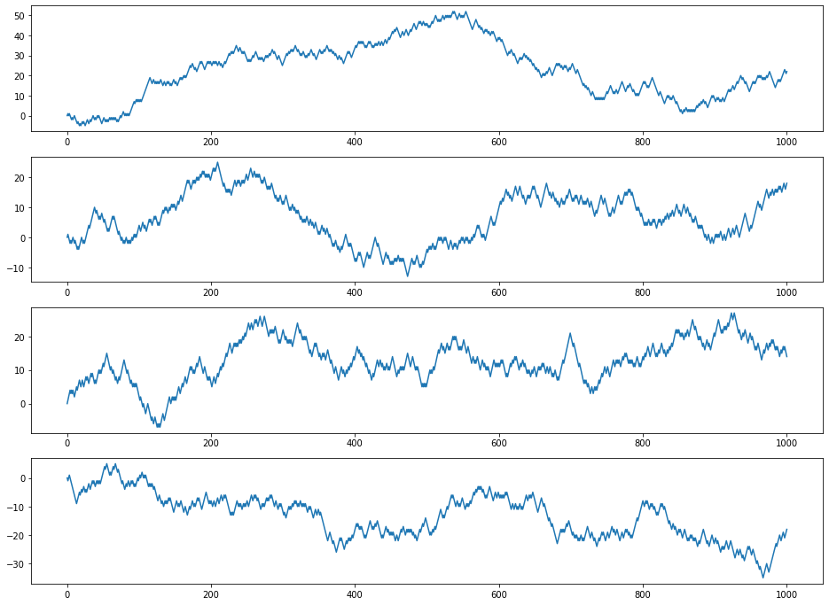
To create a simple setting where we can test our implementation of simulated annealing, we need a function that has multiple local minima. A random walk function will do the trick.
To generate a random walk, we simply need to start at an initial position, flip for a coin for whether we go up or down, and repeat. Here’s how that looks like in Python:
import numpy as np

# a function that generates a random walk within a given range
def random_walk(range_, num_points, initial_y=0):
    x_coordinates = np.linspace(*range_, num_points)
    y_coordinates = [initial_y]

    for x in x_coordinates[1:]:
        up = np.random.random() < 0.5
        if up:
            y_coordinates.append(y_coordinates[-1] + 1)
        else:
            y_coordinates.append(y_coordinates[-1] - 1)

    return x_coordinates, y_coordinates
The function we’ll be trying to optimize is one that returns the corresponding y for a given x. Let’s create a function that generates that function for a set of coordinates.
def random_walk_function(x, y):
    dic = dict(zip(x, y))
    return lambda x: dic[x]
Generate and visualize a few random walks:
import matplotlib.pylab as plt

num_walks = 4
x_min, x_max = (0, 1000)
num_points = 1001

walks = []
for i in range(num_walks):
    x, y = random_walk((x_min, x_max), num_points)
    walks.append((x, y))

fig, ax = plt.subplots(num_walks)
fig.set_size_inches(16, 12)

for i in range(num_walks):
    ax[i].plot(*walks[i])
Here’s how the output should look like:

Create a random walk function to optimize:
x, y = random_walk((x_min, x_max), num_points)

function_to_optimize = random_walk_function(x, y)
Next, we should implement our SearchState, which stores a position along the x axis. The energy of a given state is simply the value of our random walk function at the given x. To generate a neighbor, we randomly sample a new value of x that is less than 50 away (in either direction) from the current x.
class SearchState:
    def __init__(self, x):
        self.x = x

    def Energy(self):
        return function_to_optimize(self.x)

    def Neighbor(self):
        next_x = max(self.x + 50 - randint(0, 101), x_min)
        next_x = min(next_x, x_max)
        return SearchState(next_x)
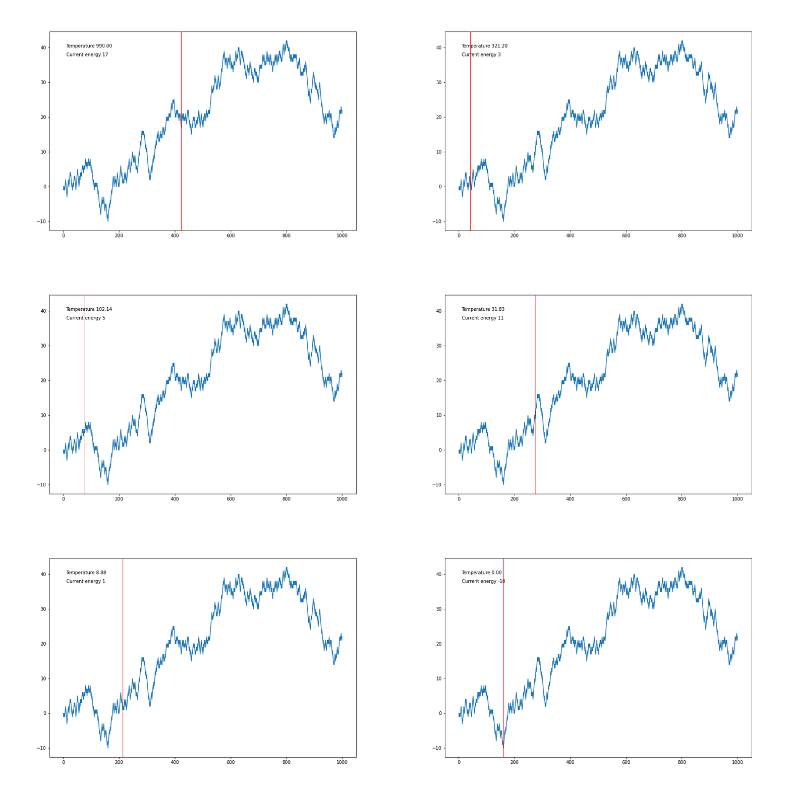
Visualizing the optimization process
We can now actually run simulated annealing on the random walk function we generated:
initial_state = SearchState(500)
best_state, history = SimulatedAnnealing(initial_state)
Let’s visualize the search process:
from matplotlib.artist import Artist
import matplotlib.animation as animation

change_history = []

for i in range(1, len(history)):
    if history[i].state != history[i-1].state:
        change_history.append(history[i])

fig,ax = plt.subplots()
fig.set_size_inches(12, 8)
ax.plot(x, y, label='function_to_minimize')
vl = ax.axvline(0, ls='-', color='r', lw=1, zorder=10)

text_temp = ax.text(10, 40, f"Temperature {change_history[0].temperature:.2f}")
text_energy = ax.text(10, 37.5, f"Current energy {change_history[0].energy}")

refresh_period = 100

def animate(i, vl, change_history, text_temp, text_energy):
    vl.set_xdata(change_history[i].state.x)
    text_temp.set_text(f"Temperature {change_history[i].temperature:.2f}")
    text_energy.set_text(f"Current energy {change_history[i].energy}")
    return vl


ani = animation.FuncAnimation(
    fig,
    animate,
    frames=len(change_history),
    fargs=(vl, change_history, text_temp, text_energy),
    interval=refresh_period
)
plt.show()

ani.save("visualization.gif", writer='imagemagick',fps=30)
And voilà
